Road to Clustered Hashing: Robinhood Hashing Revisioned
Introduction
I’ve recently been tasked to optimize the memory usage of a real time application (zeek.org). This application captures network packet and drives a lot of scripts that use dictionaries. Under certain stress tests it has created around a million dictioniaries in a matter of minutes. All of sudden how efficient the dictionary uses memory matters a lot to the overall application’s memory consumption.
Unsurprisingly the dictionary is implemented as chain-linked hash table. Why is chained hash table so popular in practice? Let’s step back a little to start from the motivation to have a hash table and see what led us here and see if we can do better.
Speed up Lookup
One of the fundamental funcionality in software is lookup. To speed up the lookup is an important goal.
Unsorted List
For a list of N items, the worst time used to look up a specific item is O(N). You basically look at them one by one. You cannot do worse than that. The items don’t have to be in order, so insert happens at the end as append so insert takes O(1). Remove takes the same as lookup O(N), because you need to find it first in O(N). To remove it, you move the last item to occupy the spot and shrink list by one. The items don’t have to use more space than necessary to store them.
Lookup: O(N)
Insert: O(1)
Remove: O(N)
Space : O(N)
Now we want to do better in lookup. Considering in computer science (and in every aspects of real life), there’s no free lunch. We have to see what can we sacrifice to speed up the lookup.
Sorted List
If we sacrifice time used in insert a bit, we can keep the list in order. You can use binary search for lookup in O(lgN) time. For insert, we first need to find the right position, same as lookup in O(lgN); then we need to shift all items larger than the new item by one to the right to make room for it, and that’s O(N). Remove is similar to insert, you need to find the item first in O(lgN) time, and then you need to shift left all items on the right of the position by one.
Lookup: O(lgN)
Insert: O(lgN) + O(N) = O(N)
Remove: O(lgN) + O(N) = O(N)
Space : O(N)
Wait, you’d think, insert and remove can be as fast as O(lgN) if we use single link list. But can you do binary search in an sorted link list? You simply have to look one by one. This solution is worse than the basic unsorted one in every aspect. And don’t forget, with link list, you use more space, as pointers occupy space, not small, 8 bytes each. We will revisit this later.
So keep list in order improves lookup greatly, but with heavy sacrifice on insert and remove. Is this a bad idea at all? Not necessarily. If you have a dictionary you insert once, never remove it, then most of the time is lookup. It is still a sensible solution.
Binary Search Tree (BST)
The next idea is to sacrice space. If adding one pointer on the item doesn’t work, How about adding two? If each item contains two pointers, we can maintain it as a binary search tree. The idea of BST is to keep items sorted, but in a special binary tree form. Lookup can perform binary search just like sorted list, but insert and remove are almost as fast as lookup. After finding the item or position, you don’t need to shift items back and forth. You simply change pointers to insert and remove, which takes almost constant time. Assume the binary tree is balanced because a variation of the BST, red black tree, can keep the tree balanced with a small price (lgN swaps).
Lookup: O(lgN)
Insert: O(lgN)
Remove: O(lgN)
Space : O(N)
This is good, isn’t it? Not so fast. As each item now requires two pointers, and each pointer is 8 bytes in 64bit CPU system, each item consumes 16 extra bytes. Suppose average item size is S, we have D=(8+8+S)/S. The space is actually O(DN). Theorectically O(DN) = O(N), but in reality you still uses D times memory than necessary. For an integer of 4 bytes, D=5. That’s a lot of memory than necessary.
Doesn’t indirection of pointers consume computer time too? For each item, you have to follow its pointers to another item. Suppose read item takes x amount of time, and load extra pointer take y amount of time, lookup actually takes O(lg((x+y)/xN) = O(lg(CN)) = O(lgC+lgN), given C=(x+y)/x. When x is small, such as read an 4-byte integer, load 8-byte takes at least same amount of time. So you could easily double the lookup time. It can be even worse… When items approach certain large counts, random pointers cause cache misses: the item pointed to is not in the current cache and CPU needs to reload it from the RAM. This is very costly. We will revisit it later. So the acutally binary search tree performance is:
Lookup: O(lgCN) = O(lgC + lgN)
Insert: O(lgCN) = O(lgC + lgN)
Remove: O(lgCN) = O(lgC + lgN)
Space : O(DN)
Sacrifice in insert and remove to the extreme make lookup as fast as O(lgN). To go further, we only have space to sacrifice. If we leave spaces among items on purpose, can we do better on lookup? Yes we can! Here comes in picture: hash table.
Hash Table
For a item with a key, we calculate an integer called hash through a hash function H: hash = H(key). We allocate a table with table_size a few times larger than item count. We then map hash to the index of the table called bucket through another map function M: bucket = M(hash, table_size). We then directly store item on position bucket, as shown below:
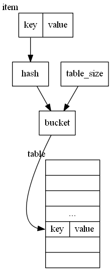
To lookup item, we do the same: hash=H(key), bucket=M(hash, table_size) table[bucket] is the item. Insert and remove are the same. find the bucket, then put to position or remove from the position (special mark). so,
Lookup: O(1)
Insert: O(1)
Remove: O(1)
Space : O(DN)
1/D is called load factor, which is usually 30-50%. So D is 2x - 3x N. For a small item such as integer, the space is even smaller than BST!
Sacrificing the space a few times makes lookup, insert and remove to be as fast as possible and ultimate goal is achieved?
Not so fast.
What if two items with K1 and K2, after function H, reaches the same hash?
H(K1) == H(K2)? With the same hash, both items find the same bucket. Follow the previous logic item 2 will overwrite item1 on insert. Even if two hashes are different, H(K1) != H(K2), mapping hash to bucket can still result in same bucket: M(H(K1), table_size) == M(H(K2), table_size).
The conflict is unavoidable. Conflict resolution is the key to implement hash tables.
Hash Table Conflict Resolution
Chain Conflicts Together
Pointers seem to be the solution to many problems. Like the binary search tree, we use indirection to link certain items together. As shown below, instead of puting item directly in the table, we put a pointer in the table, which points to a single link list. Single link list holds all the items of the same bucket. In the following diagram:
H(key) = key, H() is identity function, just for illustration only
M(hash,table_size)=hash%table_size, M is frequently used simple mapping function: mod where table_size=10
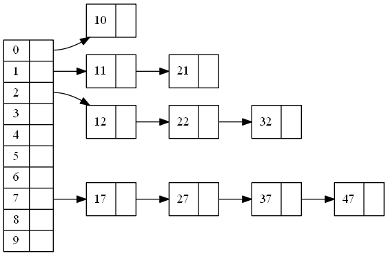
For example,
11: M(H(11),10) = M(11,10) = 11%10 = 1 and
21: M(H(21),10) = M(21,10) = 21%10 = 1
Basically the least significant decimal digit is the bucket of the key.
Both end up in the same bucket so they are chained together. With a good hash fucntion H and a reasonable table_size, sometimes with a good mapping function M, the average length(L) of the chain-link is small.
To lookup, we first map key to bucket, and then go through the single link list one by one. As pointer is involved, It takes O(cL) time. C=(pointre-read-time + item-read-time) / item-read-time. For item < 8 bytes, C>=2.
To insert, we first lookup to see if it already exists. If it does, then return or overwrite the item on spot. It takes O(CL). If it doesn’t, we add it to the head in constant time. It also takes O(CL).
To remove, we first lookup to see if it exists. If it doesn’t, then return. It takes O(CL). If it does, remove it by chaining the previous item to the next item. (Single Link List Algorithm) It also takes O(CL).
For each item with size S, it uses one extra pointer, 8 bytes. It also uses the whole extra table to store heads of single link list. Table_Size = DN, D is usually 2-3. For each item we use S+8+8D bytes. let E=(S+8+8D)/S, we use O(EN) spaces.
Lookup: O(CL)
Insert: O(CL)
Remove: O(CL)
Space : O(EN)
As L is usually < 2, this is reasonable fast.
This seems to be the perfect solution, what could be the possible downside?
The space could be. For an integer item, S=4, D=2 => E=7; for a typical 8-byte item (items are pointers), S=8, D=2 => E=4. We typically use 4x necessary memory.
constant C is also a potential cause of concern. In normal cases, C=2 is very reasonable. But when N approaches to 1 million, cache misses happen more frequently, C could even double to 4.
So what’s the reasonable next step? Well, Obviously, While maintainng the performance, to remove pointers.
Open Addressing Hash Table
Without chaining conflicts together, the only other option is to find another bucket. The process of finding another empty spot is called probing. To insert an item while its bucket is taken, there are two ways.
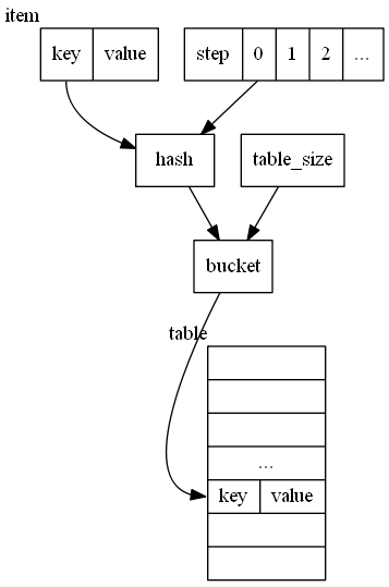
Appy a step parameter on hash function
We can also apply a step parameter directly on hash function H:
hash = H'(key,i)
where i starts from 0 forward. So
then expected position (bucket) = M(H’(key,i), table_size)
It rehashes until an empty position is found. There is no upbound of i in this case.
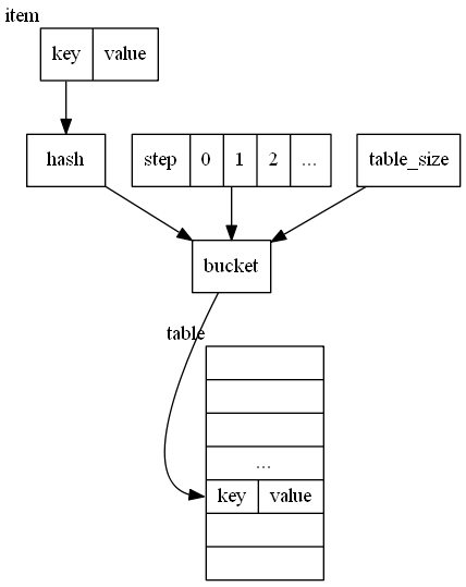
Apply a step parameter on Mapping function M
Another way is to add a step parameter in mapping function.
`M'(hash, table_size, i) = M(M(hash,table_size) + F(i), table_size)
where i starts from 0 forward. Keep increasing i until finds empty spot. A typical example of this type is linear probing.
Linear Probing
F(i) = i
If bucket of the item is not empty, Linear Probing finds the next position available. If i reaches the end of the table, it wraps around and start from 0 again. The maximum step is the table_size. It’s guaranteed the next available position will be located within table_size steps when the table is not full.
Below is an example of the open addressing hashing table with linear probing of the same elements in chained hash table.
Also noted is that the actual content of the table depends on the order of items inserted. Insert the same elements in another order renders a very different picture.
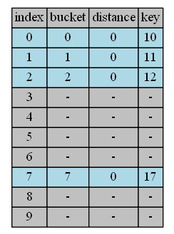
insert
insert 10,11,12,17
Item 10,11,12,17 are inserted into their buckets respectively.

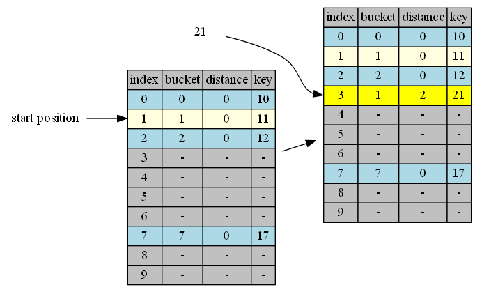
insert 21
bucket(21)=1, start from position 1.
| position | in hand | in position | action |
|---|---|---|---|
| 1 | 21, distance = 0 | 11, distance = 0 | continue |
| 2 | 21, distance = 1 | 12, distance = 0 | continue |
| 3 | 21, distance = 2 | empty | insert & done |
insert 22
bucket(22)=2, start from position 2.
| position | in hand | in position | action |
|---|---|---|---|
| 2 | 22, distance = 0 | 12, distance = 0 | continue |
| 3 | 22, distance = 1 | 21, distance = 2 | continue |
| 4 | 22, distance = 2 | empty | insert & done |
insert 27
bucket(27)=7, start from position 7.
| position | in hand | in position | action |
|---|---|---|---|
| 7 | 27, distance = 0 | 17, distance = 0 | continue |
| 8 | 27, distance = 1 | empty | insert & done |
insert 32
bucket(32)=2, start from position 2.
| position | in hand | in position | action |
|---|---|---|---|
| 2 | 32, distance = 0 | 12, distance = 0 | continue |
| 3 | 32, distance = 1 | 21, distance = 2 | continue |
| 4 | 32, distance = 2 | 22, distance = 2 | continue |
| 5 | 32, distance = 3 | empty | insert & done |

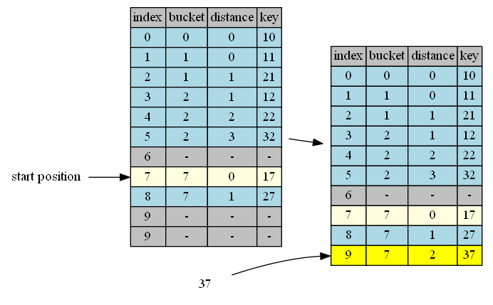
insert 37
bucket(37)=7, start from position 7.
| position | in hand | in position | action |
|---|---|---|---|
| 7 | 37, distance = 0 | 17, distance = 0 | continue |
| 8 | 37, distance = 1 | 27, distance = 1 | continue |
| 9 | 37, distance = 2 | empty | insert & done |
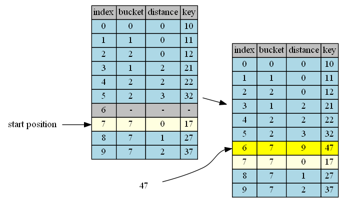
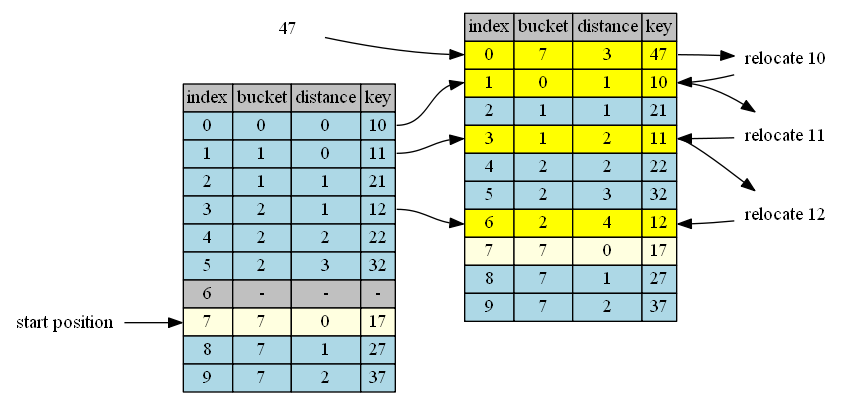
insert 47
bucket(47)=7, start from position 7.
| position | in hand | in position | action |
|---|---|---|---|
| 7 | 47, distance = 0 | 17, distance = 0 | continue |
| 8 | 47, distance = 1 | 27, distance = 1 | continue |
| 9 | 47, distance = 2 | 37, distance = 2 | continue |
| 0 | 47, distance = 3 | 10, distance = 0 | continue |
| 1 | 47, distance = 4 | 11, distance = 0 | continue |
| 2 | 47, distance = 5 | 12, distance = 0 | continue |
| 3 | 47, distance = 6 | 21, distance = 2 | continue |
| 4 | 47, distance = 7 | 22, distance = 2 | continue |
| 5 | 47, distance = 8 | 32, distance = 3 | continue |
| 6 | 47, distance = 9 | empty | insert & done |
lookup
Lookup starts with bucket and ends on the item found, an empty item, or loop through the whole table (reach table_size after wraparound).
lookup performance is highly deteriorated by too many tombstones as result of remove.
remove
The removed items has to be marked by tombstone in order not to stop lookup prematurely. If the removed item becomes empty item, the lookup stops and may not find some items inserted after the removed items.
The tomstoned item is treated the same as empty item during insertion.
The tomstoned item is treated as a no-match item during lookup.
To show how each item ends up, the table does not resize up (load factor=1) on purpose. When load factor < 1, the longest distance, table_size, will likely not be reached. However, as you can see, the distance grows dramatically when the table is getting pretty full. In the extremely case, lookup of item 47 has the worst performance of O(N).
However, on the other hand, the memory is most efficiently used.
Uncertainties
While saving space, open address hash table adds some uncertainties.
-
There’s a great deal of variance in lookup. Lookup in Chained Hash Table for an item that exists or not, takes an upbound of the most conflicts on the position. Unlike Chained Hash Table, Open Address Table usually has a great deal of variance in steps to find an item. The number of steps has little to do with the conflicts on that specific item. The same item may be found in one try, or it may be found in 1000+ tries. Even worse, lookup of an item that’s not in the table takes most of time as it ends when an empty position is found.
-
There’s no clear invariant on the data structure. Chained Hash Table has a nice property: Every item in the chain belongs to the bucket it maps to from key
M(H(key), table_size). Before and after every operation you can put assertions on this property to make sure the operation is correctly performed. Items in Open Addressing Hash Table, either appear at its bucket, or they appear anywhere in the table. This makes some operations hard to verify.
What can we do to improve? Just as the thought process goes along the way, to make lookup more consistent, we have to think what we can sacrifice. From unsorted list to sorted list, we sacrifice the performance of insert for a better performance of lookup. From sorted list to binary search tree, we sacrifice space to improve insert and delete. From BST to Chained Hash Table we sacrifice more space to improve on lookup, insert and remove. From Chained Hash Table to Open addressing Hash Table we try to recoup some space back while maintain performance of lookup, insert and remove. To improve the uncertainty of lookup, is there anything left that we can sacrifice?
As it turns out, there is. To improve the worst case lookup, we can sacrifice best case lookup.
Robinhood Hashing
When we insert an item into hash table, we look for an empty position to put it in. Ideally the position is at its bucket. But if not, we keep looking for other positions via differnet strategies. Doing so we actually follow a hidden rule that when an item is in the table, we don’t change its position anymore. This rule can lead to a really bad position when the table is pretty full and an empty position is far away.
The alternative is to adjust the position of existing items if necessary during insertion. When looking for empty positions to insert the new item, Robinhood Hashing compares the to-be-inserted item distance from its bucket if it’s inserted on the current position. If it’s longer than the distance of the item occupying the current position. the to-be-inserted item swaps the item out and takes the position. Then it continues to look forward to insert the swapped out item. When it reaches the end of the table, it wraps around from beginning.
Robinhood Hashing can be applied to any open addressing hash item idea. Let’s investigate how it applies to simplest case: linear probing.
We take the same table size and insert the same items as in previous Open Hashing table: insert 10,11,12,17,21,22,27,32,37,47 to hash table of size 10.
insert
insert 10,11,12,17
Item 10,11,12,17 are inserted into their buckets respectively, which is the same as in Open Address Linear Probing.
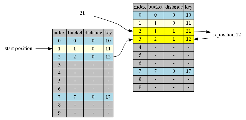
insert 21
bucket(21)=1, start from position 1.
| position | in hand | in position | distance comparison (in position vs in hand) |
action |
|---|---|---|---|---|
| 1 | 21, distance = 0 | 11, distance = 0 | same | continue |
| 2 | 21, distance = 1 | 12, distance = 0 | shorter | swap |
| 3 | 12, distance = 1 | empty | insert & done |
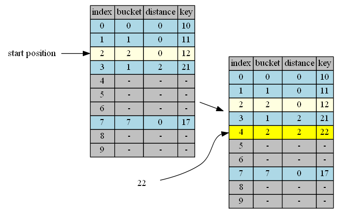
insert 22
bucket(22)=2, start from position 2.
| position | in hand | in position | distance comparison (in position vs in hand) |
action |
|---|---|---|---|---|
| 2 | 22, distance = 0 | 21, distance = 1 | longer | continue |
| 3 | 21, distance = 1 | 12, distance = 1 | same | continue |
| 4 | 12, distance = 2 | empty | insert & done |

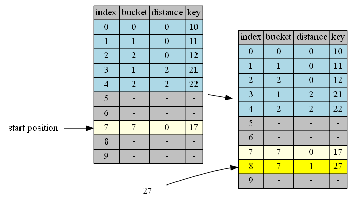
insert 27
bucket(27)=7, start from position 7.
| position | in hand | in position | distance comparison (in position vs in hand) |
action |
|---|---|---|---|---|
| 7 | 27, distance = 0 | 17,distance=0 | same | continue |
| 8 | 27, distance = 1 | empty | insert & done |

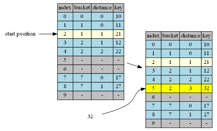
insert 32
bucket(32)=2, start from position 2.
| position | in hand | in position | distance comparison (in position vs in hand) |
action |
|---|---|---|---|---|
| 2 | 32, distance = 0 | 21,distance=1 | longer | continue |
| 3 | 32, distance = 1 | 12,distance=1 | same | continue |
| 4 | 32, distance = 2 | 22,distance=2 | same | continue |
| 5 | 32, distance = 3 | empty | insert & done |
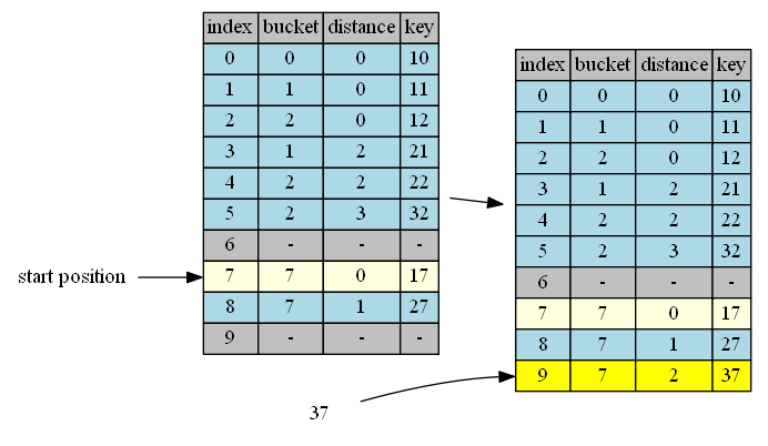
insert 37
bucket(37)=7, start from position 7.
| position | in hand | in position | distance comparison (in position vs in hand) |
action |
|---|---|---|---|---|
| 7 | 37, distance = 0 | 17,distance=0 | same | continue |
| 8 | 37, distance = 1 | 27,distance=1 | same | continue |
| 9 | 37, distance = 2 | empty | insert & done |
insert 47
bucket(47)=7, start from position 7.
| position | in hand | in position | distance comparison (in position vs in hand) |
action |
|---|---|---|---|---|
| 7 | 47, distance = 0 | 17,distance=0 | same | continue |
| 8 | 47, distance = 1 | 27,distance=1 | same | continue |
| 9 | 47, distance = 2 | 37,distance=2 | same | continue |
| 0 | 47, distance = 3 | 10,distance=0 | shorter | swap |
| 1 | 10, distance = 1 | 11,distance=0 | shorter | swap |
| 2 | 11, distance = 1 | 21,distance=1 | same | continue |
| 3 | 11, distance = 2 | 12,distance=1 | shorter | swap |
| 4 | 12, distance = 2 | 22,distance=2 | same | continue |
| 5 | 12, distance = 3 | 32,distance=3 | same | continue |
| 6 | 12, distance = 4 | empty | insert & done |
Robinhood table structures
If you look at the structure of items in Robinhood table, you can easily spot its characteristics: unlike the normal open address table, items of the same bucket are clustered together in Robinhood table.
remove
tombstone.
One way to remove is like the open address table, to mark it as tombstone. Tombstone makes removal very fast but at an expense of lookup.
However, tombstone has another huge downside in Robinhood hashing. It wastes a lot of space. Because items in Robinhood table cluster together, the tombstone within the specific cluster has to be considered the tombstoned item within that cluster. That means, during insert, only the item belonging to that specific cluster can use this tombstone’d space. And the probability is very small of this reuse case.
shift items up.
When an item is removed, we shift the items behind this newly emptied position up by one, if the shift reduces distance of the item, until it reaches another empty position (an empty position’s distance cannot be reduced.). This is suggested by Sebastian Sylvan in More on Robin Hood Hashing
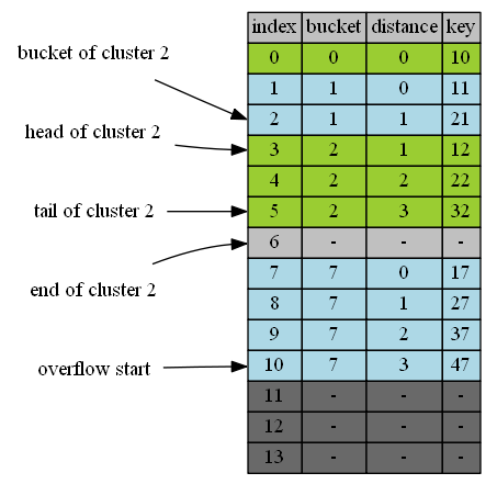
Clustered Hashing
Since Robinhood Hashing idea applies to all methods of Open Addressing Hashing, the special clustered property when it applies to Open Addressing Linear Probing is rarely explored explicitly. Even Sebastian Sylvan never mentioned it. If we take the cluster property out of the context of Robinhood Hashing and develop on it, We will see that all of sudden it addresses the second uncertainty of Open Addressing Hashing: It now has an simple invariant: All items of the same bucket clustered.
Let’s take the cluster idea a bit further: We add overflow positions at the end of the table to avoid wrap-arounds. With the condition, we have another invariant: Clusters of bigger buckets always resides after the clusters of smaller buckets. ie. The clusters are in order of buckets. This small variation simplifies a few complex algorithms and paves the way for more complex algorithms on it.
So what’s Clustered Hashing?
- The flattened version of Chained Hashing.
- An Open Addressing Hashing. It puts items directly in the table.
- An Robinhood Hashing. It adjusts existing items while inserting new items.
Clustered Hashing also sacrifices constant property during deletion and lookup.
- It adjusts other existing items while deleting items.
- It adjusts existing items during lookup when incremental sizing is implemented.
Heres the visual comparison of Chained and Clustered Hashing:
| Chained Hashing | Clustered Hashing |
|---|---|
|
 |
I’ll discuss the details of Clustered Hashing operation in the next post: Clustered Hashing: Basic Operations
Lessons Learned
“There can be no progress, no achievements, without sacrifice, and a man’s worldly success will be in the measure that he sacrifices.” -James Allen, As a Man Thinketh.