Clustered Hashing: Basic Operations

Introduction

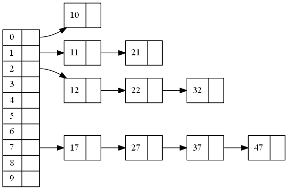
Clustered Hashing is the flattened version of Chained Hashing. Chained Hashing links items of the same bucket together by pointers. Clustered Hashing clusters items of the same bucket together directly in the hash table.

Here’s the visual comparison of Chained and Clustered Hashing:

Chained Hashing	Clustered Hashing

The reasoning that leads to this data structure is here: Clustered Hashing.

Table Size & Map Function: Fibonacci Hashing

Before getting into the details of the Clustered Hashing, let’s discuss the table size and mapping mechanism first. Normally each index in hash table is a bucket. Keys are hashed and mapped into [0,table_size) range.

To get the bucket from key, we use

bucket=M(H(key),table_size)

Map function M usually is a single mod function below:

M(hash,table_size) = hash % table_size.

There are a few issues with this map function:

• table_size needs to be a prime to make it really effective. And the increasingly large primes are hard, and expensive to find. When we compromise with just an odd large integer, the mapping function may perform worse. It results in more collisions.
• hash % table_size looks very simple, but is expensive to calculate. It uses division, which involves loops.
• the bucket mapping depends heavily on the hash function. A bad hash function, for example, an integer identity function, may cause a lot of collisions.

Fibonacci Hashing is a map function from hash to a range of (0, table_size). It solves all three issues above and adds one more benefit in the case of incremental resizing, to be discussed in the next post: Clustered Hashing: Incremental Resize

• table_size is always 2^N. so table_size is represented by bits N
• bucket = M(hash,N) = lower N bits of (hash * 2^64 / phi) , phi = Golden Ratio = 1.618033987…

2^64/phi = 11400714819323198485

You can find details about Fibonacci Hashing here: Malte Skarupke, Fibonacci Hashing: The Optimization that the World Forgot

hash_t FibHash(hash_t hash)
{
    hash *= 11400714819323198485llu; //2^64/phi
    return hash;
}

int BucketByHash(hash_t h, int log2_table_size)
{
    if( !log2_table_size )
        return 0;
    int m = 64 - log2_table_size;
    hash_t hash = FibHash(h);
    hash <<= m;
    hash >>= m;
    return hash;
}

int BucketByKey(Key key, int log2_table_size)
{
    return BucketByHash(Hash(key), log2_table_size);
}

To keep table simple and avoid table wrap-around, an overflow area is attached to the end of the table. Now the table has an advertised size of table_size, represented by log2_table_size, and an internal table size.

internal_table_size = table_size + overflow_size.
overflow_size = log2(table_size) + C, where C is a constant.

Buckets() returns table size. Capacity() returns internal table size

int Buckets()
{ 
    return 1<<log2_buckets;
}

int Capacity()
{ 
    return (1<<log2_buckets) + log2_buckets;
}

In chained hash table, the bucket is the position, ie. the index of the table. In clustered hashing table, they are different. Bucket is what hash function is mapped to the range (0, table_size). And position is the index of the table in the range (0, table_size + overflow size).

Item/Entry Attributes

Each entry in the table has 3 attributes:

name	description
position	position, index in the table the item is in.
bucket	bucket of the item, or the perfect position of the item. b = M(H(key),table_size), where M is the Map function to map hash to the range of [0, table_size-1], H is the hash function of key.
distance	distance of the item’s actual position from its bucket. distance >= 0 When the item is in its expected bucket position, the distance = 0. Likely the item is off from its bucket because its bucket positon is occupied by another item. A special distance = -1 is used to identify an empty item.

Items in Clustered Hashing Table satisfies the following equation:

position = bucket + distance

So we only need to maintain a distance attribute for the item and derive bucket from it by

bucket = position - distance

int BucketByPosition(int position)
{
    return position - table[position].distance;
}

Structure of the table

Basic Properties:

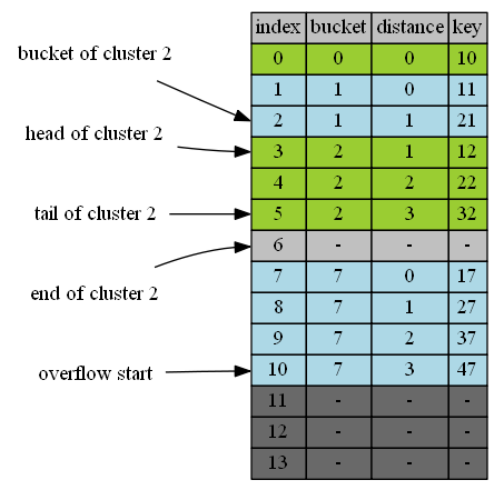
1. (B1-Cluster) Items are arranged in clusters. Items of the same bucket belong to the same cluster. cluster 7 has 4 items 17,27,37,47 all of bucket 7.
2. (B2-Bucket) Cluster is located at or after its bucket. Clusters of items in bucket b is called cluster b. For example in the diagram, cluster 1 starts from postion 1, its bucket(1). Cluster 2 starts from position 3, after its bucket(2).
3. (B3-Order) Clusters are arranged in the order of its bucket. For example, Cluster 1 is before cluster 2.
4. (B4-Position) Each cluster is located at its closest possible position to its bucket while maintaining cluster properties 1,2, and 3.

Derived Properties:

1. (D1 - No Gap Before) No gaps between bucket of cluster and its head. If it had, we could have shifted the cluster b up to reduce the distance of the cluster b. The shifted arrangement has closer distance from its bucket. This conflicts to Basic Property 4.
2. (D2 - No Gap Inside) No gaps inside the cluster. If it had, we could have shifted the item of the cluster right after that gap up to improve its distance. This makes the arrangement conflict to Basic property 4.
3. (D3 - Non-negative Distance) Distance maintained in the item is non-negative. Each item in the cluster maintains the distance from its actual position to its perfect position (bucket). Since clusters reside at or after its perfect position, the distance is always non-negative.
4. (D4-Continuous Distance Inside) Distances of items in the same cluster are in continuous ascending order. Since items of the same cluster are contiguous, the distances are continuous. For exampe, cluster 2 has 3 items. The head of the cluster is 12, with distance of 1. It contains 3 items with distances of 1,2, and 3.

The operations are all based on these 4 basic and 4 derived properties.

The hash is saved with key-value pair in the table entry here. When table size grows, it saves time to recalculate hash and map hash to another range. It also saves time on comparison of keys as it can now compare hash first. Only when hash does match it compares key. If space optimization is more important the extra time savings. We can take hash out.

distance is put as 2-byte unsigned integer directly in the entry. If extra space savings is necessary, we can put distance into a separate array with table array to have one byte distance and can possibly take 2-byte distance when it is necessary. We usually require entries are in multiples of 8 to keep it alligned to perform fast. With Clustered Hashing, distances are evenly distributed and very rarely go over log2(N). A dictionary of 1 million entries usually has distances less than 20.

template<class Key, class Value> 
class Dictionary
{
    struct Entry
    {
        Key key;
        Value value;
        hash_t hash;
        uint16 distance;

        bool Empty(){return distance == 0xFFffFFff;}
        void SetEmpty() {distance = 0xFFffFFff;}
        bool Equal(const Entry& other){ return hash == other.hash && key == other.key;}
        bool operator==(const Entry& other){ return Equal(other); }
        bool operator!=(const Entry& other){ return !Equal(other); }
        Entry(Key key, const Value value, uint32 hash, uint16 distance): key(key), value(value), hash(hash), distance(0){}
    };

    Entry* table;
    char log2_buckets; //2^log2_buckets is the table_size.
    int num_entries;

    hash_t Hash(const Key& key) const;
    int BucketByHash(uint32 hash, int log2_table_size) const;
    int BucketByKey(Key key) const;
    int Buckets() { return 1<<log2_buckets;}
    int Capacity() { return (1<<log2_buckets) + log2_buckets;}
};

Lookup

Find the head and tail of the cluster b

• Based on B2-Bucket, we know the head of cluster is at or after b. So the search range starts from b.

• Based on B3-Order, From b on

  • we may first see partial or full of a cluster smaller than b0.
  • We then may see other full clusters b1, b2, …, b-1.
  • we then may see the cluster of b.
  • no gaps between b and the tail of cluster b.
  • we then may see other full clusters b+1, b+2, …

Solution:

1. From b on, the first position with bucket of b is the head of the cluster b if it exists.
2. From b on, the last position with bucket of b is the tail of the cluster b if it exists.
3. When we reach next cluster (B3-Order), or an empty position(D1&D2 - No Gap), or the end of the table. We know cluster b doesn’t exist.

For example, head of cluster 2 is 3, the first position at or after 2 whose bucket is 2. The tail of cluster 2 is 5, the last position whose bucket is 2.

If we don’t find positions of bucket b before we reach the end of table, find empty space or the cluster greater than b, we know cluster b doesn’t exist.

For example, when we look for head of cluster 4. Starting from position 4, we first see part of cluster 2. We then see empty space of position 6. If we had cluster 4, it must reside before empty space, ie 6. So we konw cluster 4 doesn’t exist.

int HeadOfClusterByBucket(int bucket) const
{
    int i = bucket;
    for(; i < Capacity() && !table[i].Empty() && BucketByPosition(i) < bucket; i++)
        if( BucketByPosition(i) == bucket)
            return i;
    return -1;
}

int TailOfClusterByBucket(int bucket) const
{
    int end = EndOfClusterByBucket(bucket);
    if( end - 1 >= 0 && !table[end-1].Empty() && BucketByPosition(end - 1) == bucket )
        return end - 1;
    return -1;
}

int Dictionary::EndOfClusterByBucket(int bucket) const
{
    int i = bucket;
    while( i < Capacity() && !table[i].Empty() && BucketByPosition(i) <= bucket)
        i++;
    return i;
}

Find the Head, Tail, End and Offset of the cluster position p belongs to

This is straight-forward. As we know items of the cluster stay together, we only need to look up and down. The farthest position up with the same bucket of position is the head of my cluster and the farest position down with the same bucket of position is the tail of my cluster.

int HeadOfClusterByPosition( int position) const
{
    int bucket = BucketByPosition(position);
    int i = position;
    while( i >= bucket && BucketByPosition(i) == bucket )
        i--;
    return i == bucket ? i : i + 1;
}

int TailOfClusterByPosition(int position) const
{
    int bucket = BucketByPosition(position);
    int i = position;
    while( i < Capacity() && !table[i].Empty() && BucketByPosition(i) == bucket )
        i++;
    return i - 1;
}

int EndOfClusterByPosition(int position) const
{
    return TailOfClusterByPosition(position)+1;
}

int OffsetInClusterByPosition(int position) const
{
    int head = HeadOfClusterByPosition(position);
    return position - head;
}

Lookup specific key

Because if cluster b exists, from position b to the tail of cluster b, the table items are contiuous without gaps. Starting from b we loop through it until we find a gap(empty position), a larger cluster, or end of table. When cluster is right we compare hash and key to find the match.

The reason to have one extra wrapper of LookupIndex() is to handle lookup and its optimization during hash table resizing. nt LookupIndex(Key key, hash_t hash, int* insert_position = NULL, int* insert_distance = NULL) is extended in the next post.

Value* Lookup(Key key)
{
    hash_t hash = Hash(key);
    int position = LookupIndex(key, hash);
    return position >= 0 ? &table[position].value : NULL;
}

int LookupIndex(Key key, hash_t hash, int* insert_position = NULL, int* insert_distance = NULL)
{
    if( !table )
        return -1;
    int bucket = BucketByHash(hash);
    int end = Capacity();
    return LookupIndex(key, hash, bucket, end, insert_position, insert_distance);
}

int LookupIndex(Key key, hash_t hash, int bucket, int end, int* insert_position = NULL, int* insert_distance = NULL)
{
    int i = bucket;
    for(; i < end && !table[i].Empty() && BucketByPosition(i) <= bucket; i++)
        if( BucketByPosition(i) == bucket && table[i].hash == hash && table[i].key )
            return i;
    if(insert_position)
        *insert_position = i;
    if(insert_distance)
        *insert_distance = i - bucket;
    return -1;
}

For example, Lookup(22). we look continuously from position 2. We compare bucket to locate head of cluster 2, which is position 3. We then going through the cluster 2 and find 32 on position 4.

Lookup(26), we start from position 6. Because position 6 is empty, we know immediately cluster 6 doesn’t exist. If we want to insert 26, position 6 is the position to insert.

Lookup(23), we start from position 3. Looking for head of the cluster 3 ends with position 6 as its empty. So we know cluster 3 doesn’t exist. If we want to insert 23, position 6 is the position to insert.

Insert

I1. To insert key K with bucket b. K has to be appended to the tail of the cluster.

Proof:

• B4 tells us all items are in their closest possible positions while maintaining the properties of the Clustered Hashing. So before the head of the cluster b there is no position for key of cluster b to insert. Had there been, head of the cluster b is not best positioned. So the position to insert key is at or after the head of cluster b.
• D2 tells us there are no gaps inside cluster b. So we cannot put k into a gap inside the cluster.
• So to put k in any position inside the cluster, we have to swap out the item in that position.
• B4 tells us all items are already in their best position. If we put key in and take out the item in that position, we face the same problem to insert the item in hand of the same cluster as the original key without achieving anything.
• B1 tells us items of the same cluster are together. If we can’t put the key before the head of the cluster, nor do we want to put it inside the cluster, the only option left is to put it at the end of the cluster, after tail of the cluster.

I2. To swap the item, we take out the head of the next cluster and append it to the tail of the same cluster.

Proof:

• When we insert an item, we append to the end of the cluster.
• B1 tells us items of the same bucket cluster together. If the end of the cluster b is the middle of the next cluster c, that means insertion of the item causes some items of cluster c before it. Now cluster b is mixed with the item of cluster c. This contradicts with B1. So the append position is the head of the next cluster.

I1 and I2 forms the algorithm of insertion.

We lookup first. If key is already in the table, we update the value.

If it’s not, we find the insert position p:

• If cluster b exists, p = the end (tail of cluster + 1) of the cluster b.
• If clustere b doesn’t exist, p = the end of the cluster just smaller than b (So insertion of key starts the cluster of b).
• If p is empty, we insert to that position p and done.
• If p is not emepty, it must be the head of next the cluster. we swap it with item in hand and append it to the end of its cluster.
• The process goes on until an empty position so no item is in hand after insertion.
• Adjust distances of the item in hand accordingly.

The core algorithm is implemented in InserAndRelocate(). Extra wrappers are used for adjustment during incremental resizing.

void  Insert(Key& key, Value& value){
    hash_t hash = Hash(key);
    int insert_position = 0;
    int insert_distance = 0;
    int position = LookupIndex(key, hash, &insert_position, &insert_distance);
    if( position > 0 )
    {
        table[i].value = value;
        return;
    }
    Entry entry(key, value, hash, insert_distance);
    InsertRelocateAndAdjust(entry, insert_position);
}

void InsertRelocateAndAdjust(Entry& entry, int insert_position)
{
    int last_affected_position = position;
    InsertAndRelocate(entry, insert_position, &last_affected_position);
}

void InsertAndRelocate(Entry& entry, int position, int* last_affected_position)
{
    while(true)
    {
        if(insert_position >= Capacity())
        {
            SizeUp();
            table[insert_position] = entry;
            if(last_affected_position)
                *last_affected_position = insert_position;
            return;
        }
        if(table[insert_position].Empty())
        {
            table[insert_position] = entry;
            if(last_affected_position)
                *last_affected_position = insert_position;
            return;
        }
        auto t = table[insert_position];
        int next = EndOfClusterByPosition(insert_position);
        t.distance += next - insert_position;
        table[insert_position] = entry;
        entry = t;
        insert_position = next;
    }
}

The following examples to insert items one by one from empty table with table_size = 10 and capacity = 14.

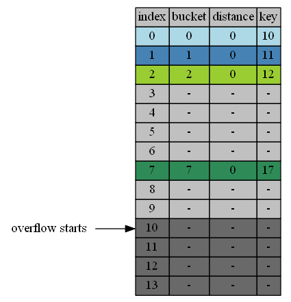
insert 10,11,12,17

The simplest case. Their individual buckets are empty.

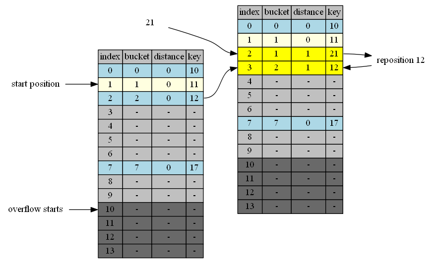
insert 21

• 21 belongs to cluster 1. Cluster 1 has only one item (11). Head and tail of Cluster 1 is 1. end of clustere 1 is position 2.
• In position 2 is 12, the head of cluster 2. end of cluster 2 is position 3. we swap 12 with 21 in hand.
• position 3 is empty. Adjustment ends.

The process can be described by the following table:

in hand	insert position	in position	cluster	end of cluster	action
21	2	12	2	3	21<->12
12	3	-	-	-	12->empty position

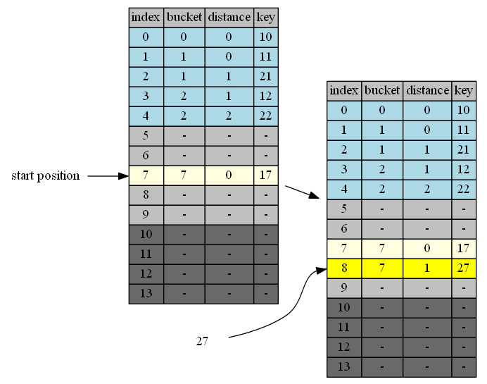
insert 27

27 belongs to cluster 7. end of cluster 7 is position 8. 8 is the first insertion position.

in hand	insert position	in position	cluster	end of cluster	action
27	8	-	-	-	27->empty position

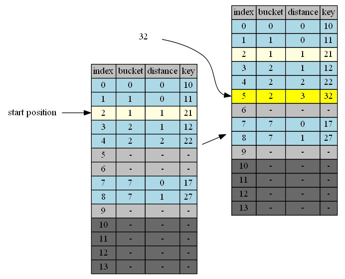
insert 32

32 belongs to cluster 2. end of cluster 2 is position 5. 5 is the first insertion position.

in hand	insert position	in position	cluster	end of cluster	action
32	5	-	-	-	32->empty position

insert 37

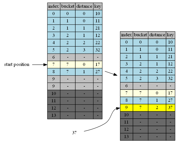
37 belongs to cluster 7. end of cluster 7 is position 9. 9 is the first insertion position.

in hand	insert position	in position	cluster	end of cluster	action
37	9	-	-	-	37->empty position

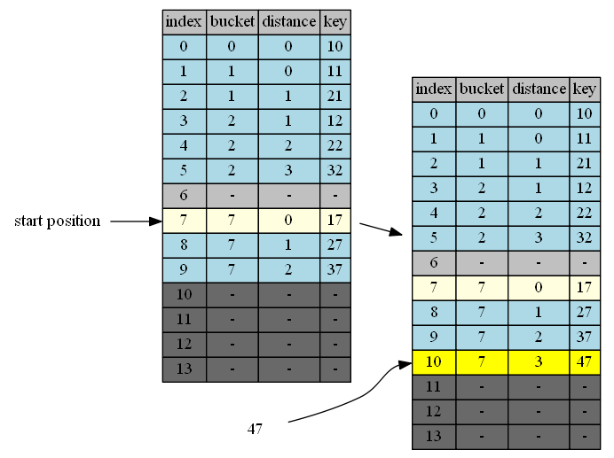
insert 47

47 belongs to cluster 7. end of cluster 7 is position 10. 10 is the first insertion position.

in hand	insert position	in position	cluster	end of cluster	action
47	10	-	-	-	47->empty position

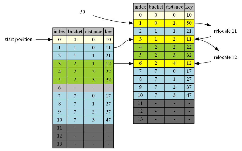
insert 50

50 belongs to cluster 0. end of cluster 0 is position 1. 1 is the first insertion position.

in hand	insert position	in position	cluster	end of cluster	action
50	1	11	1	3	50<->11
11	3	12	2	6	11<->12
12	6	-	-	-	4->empty position

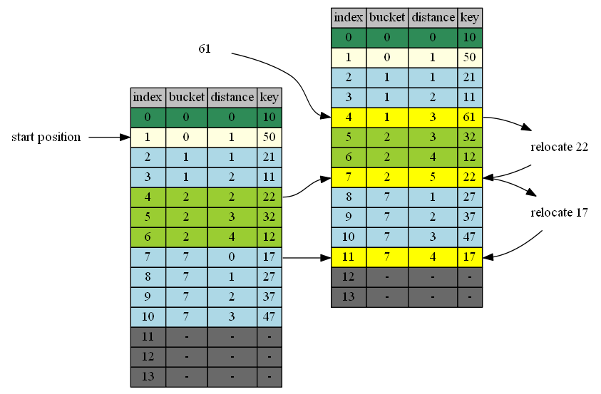
insert 61

61 belongs to cluster 1. end of cluster 1 is position 4. 4 is the first insertion position.

in hand	insert position	in position	cluster	end of cluster	action
61	4	22	2	7	61<->22
22	7	17	7	11	22<->17
17	11	-	-	-	17->empty position

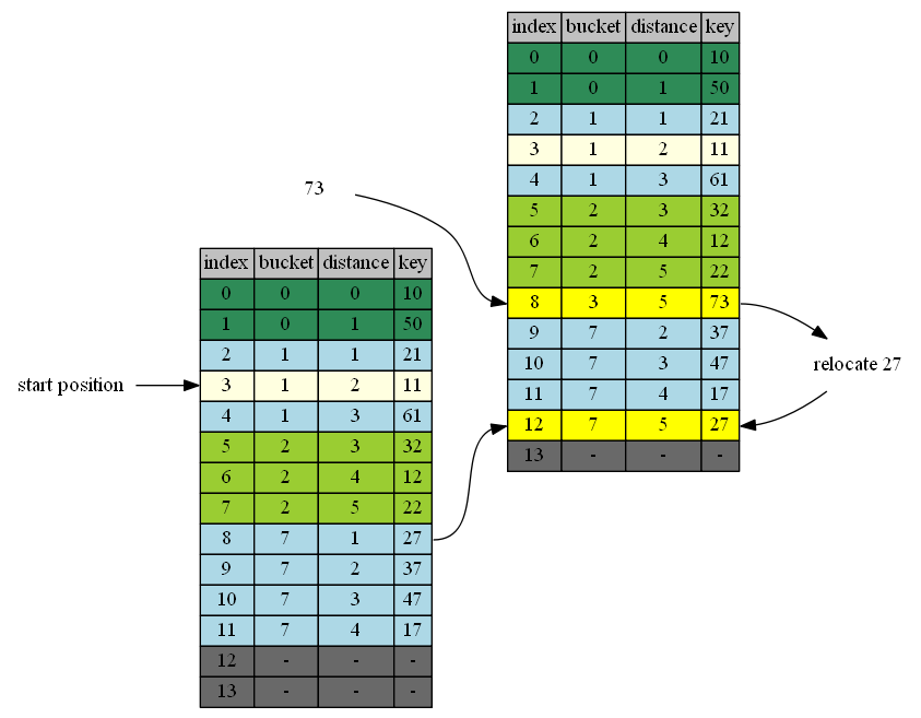
insert 73

73 belongs to cluster 3. cluster 3 doesn’t exist. End of cluster 2 (the cluster right before 3) is position 8. 8 is the first insertion position.

in hand	insert position	in position	cluster	end of cluster	action
73	8	27	7	12	73<->7
7	12	-	-	-	7->empty position

Remove

R1: D1 states no gaps exist inside the cluster. If the item at position p is inside the cluster, removal causes gap inside the cluster. we need to reduce this gap. To reduce the gap, we relocate the tail of the cluster to the position p.

R2: D2 states no gaps exist between bucket b and the head of cluster b. A gap at position p between cluster a and b needs to be reduced if it sits between b and head of cluster b. To reduce it, we move the tail of cluster b to position p. Position p becomes the new head of cluster b.

R1 and R2 forms the algorithm of removal:

1. Lookup the key, if position p is not found, it returns. Otherise empty position p.
2. If the p is the end of the table, or p+1 is also empty or the head of the next cluster b is at its bucket (distance=0). Done.
3. Find the tail of cluster b to fill position p.
4. Repeat 2 to fill new empty position at the previous tail of cluster b.

To fill the position p vacated by Remove(), the tail of cluster at p+1 is used. To fill the rest, the tail of the cluster is removed to become the head of the same cluster.

The core algorithm of remove is implemented in RemoveAndRelocate().

void Remove(Key& key)
{
    int position = LookupIndex(key, Hash(key));
    if( position < 0 )
        return; 

    RemoveRelocateAndAdjust(position);
}

Entry RemoveRelocateAndAdjust(int position)
{
    int last_affected_position = position;
    Entry entry = Remove(position, &last_affected_position);
    return entry;
}

Entry RemoveAndRelocate(int position, int* last_affected_position)
{
    Entry entry = table[position];
    while(true)
    {
        if( position == Capacity() - 1 || table[position+1].Empty() || table[position+1].distance == 0)
        {
            table[position].SetEmpty();
            last_affected_position = position;
            return;
        }
        int next = TailOfMyCluster(position+1);
        table[position] = table[next];
        table[position].distance -= next - position;
        position = next;
    }
    return entry;
}

The following examples illustrate the algorithm of remove.

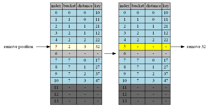
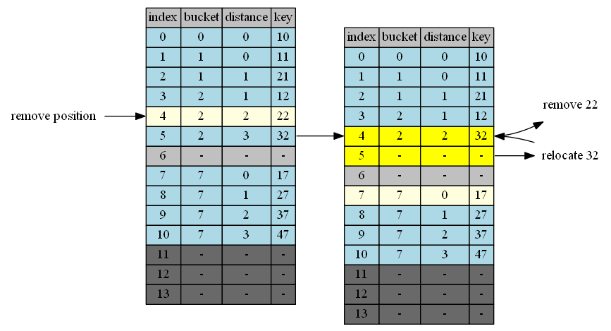
Remove 32

32 at position 5

empty position	position+1	cluster @p+1	tail of cluster	action
5	6	-	-	done

Remove 22

22 at position 4

empty position	position+1	cluster @p+1	tail of cluster	action
4	5	2	5	5->4
5	6	-	-	done

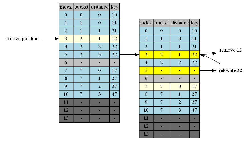
Remove 12

12 at position 3

empty position	position+1	cluster @p+1	tail of cluster	action
3	4	2	5	5->3
5	6	-	-	done

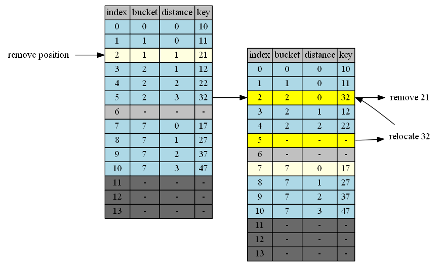
Remove 21

21 at position 2

empty position	position+1	cluster @p+1	tail of cluster	action
2	3	2	5	5->2
5	6	-	-	done

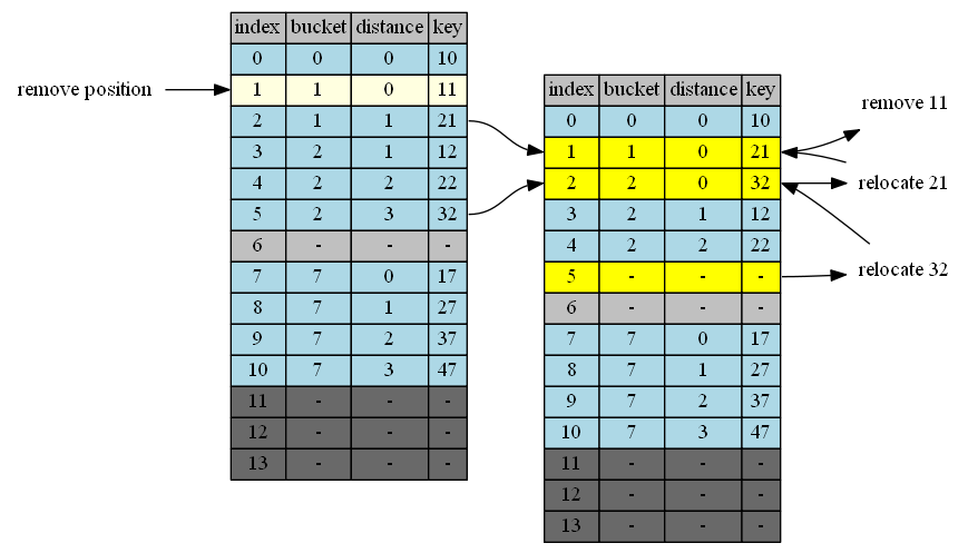
Remove 11

11 at position 1

empty position	position+1	cluster @p+1	tail of cluster	action
1	2	1	2	2->1
2	3	2	5	5->2
5	6	-	-	done

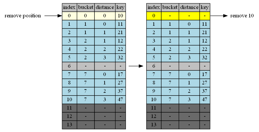
Remove 10

10 at position 0 cluster 1 is alreadly optimally located.

empty position	position+1	cluster @p+1	distance	tail	action
0	1	1	0	-	done

This post covers the basic operations on the clustered hashing table: lookup, insert and remove. This is enough for most of the use cases. However, in some real time systems, we need to spread out the time spent to resize the table. The next post focuses on this specific problem. As it turns out, Clustered Hashing has a neat solution to the incremental resizing problem. I discusses it in the next post: Clustered Hashing: Incremental Resize.

References

• Clustered Hashing
• Clustered Hashing: Incremental Resize
• Clustered Hashing: Modify On Iteration
• Sebastian Sylvan, Robin Hood Hashing should be your default Hash Table implementation
• Malte Skarupke, Fibonacci Hashing: The Optimization that the World Forgot